Executive Summary

• Medicare uses a variety of geographic adjustments to equalize payments across geographic areas in order to account for variations in operating costs.
• The two most widely used types of geographic adjustments in Medicare are the Hospital Wage Index (HWI) and the three Geographic Practice Cost Index values (GPCIs); the former is used to account for geographic variations in hospital labor costs, and the latter is used to account for geographic variations in physician practice costs.
• The accuracy and usefulness of the methods for determining both the HWI and GPCI have been questioned, as there are concerns that neither fully accounts for the geographic variation in costs of operation for hospitals, physicians, and other health care occupations.
• Both the HWI and GPCI geographic adjustments suffer from limited data and decades-old assumptions, although any update would run into political as well as policy implementation challenges.

Introduction

In 2019, Medicare reported total expenditures for Part A and B of roughly $698.6 billion.[1] The vast majority of these funds, excluding Part B drugs and medical devices, were spent through Medicare’s Fee-for-Service (FFS) system as payment to providers for individual hospital and physician services. FFS relies on a host of complex formulas to determine payment for services. These formulas seek, as closely as possible, to match payment to the true market value of a given service, as well as achieve certain policy goals (for example, to ensure better access to care in rural or impoverished areas). The formulas must take into account a host of factors: type of diagnosis, severity of diagnosis, how the diagnosis was attained, the specific treatments used for the diagnosis, the complexity of the individual treatment chosen, the bundle of services that goes along with that treatment chosen, the real cost of providing that treatment, and other factors. The cost of providing the treatment is itself influenced by multiple variables: the amount of labor and the mix of labor used in providing the treatment (potentially involving physicians, nurse practitioners, orderlies, or other providers); and the capital costs of the provider, including rent and taxes. Cost of living directly impacts the price of labor, so personnel costs vary substantially based on location. Similarly, rent and taxes vary substantially between different communities. Medicare accounts for these latter differences through geographic adjustment formulas.

This primer will explain two of Medicare’s geographic adjustment methods that account for geographically linked costs for providers: the Hospital Wage Index (HWI) and Geographic Practice Cost Index (GPCI). These two adjustment methods were chosen because of their focus on labor expenses, which are a primary cost-driver for providers. Additionally, this primer will discuss concerns surrounding the effectiveness of these two geographic adjustment methods.

Background

Geographic adjustment is the process by which Medicare adjusts compensation for providers to reflect geographic differences in labor and capital expenses. Geographic adjustment seeks to ensure that all else being equal, a provider in a high-cost area such as San Francisco or Manhattan is compensated at a similar level as a provider in a lower-cost area such as Indianapolis. Two types of geographic adjustments used by Medicare are the HWI and GPCIs. These are intended to be reimbursement tools seeking fair compensation and not policy tools seeking specific outcomes.[2] As such, this primer will not discuss certain other rate adjustments such as separate payment supports for rural hospitals that, while geographically dependent, are policy tools and not pure reimbursement tools.

In order to capture purely geographic factors of labor expenses beyond the control of providers and not also include the decisions of providers that may lead to more or less expensive care, geographic adjustments are intended to account for the price of labor, rather than the cost of labor. In the context of this primer, the cost of labor means the amount of money a given provider spends on labor, while the price of labor is the actual dollar value of the labor used to provide a medical service. Put another way, the provider can choose how many nurse practitioners or licensed practical nurses to hire – which will help determine the cost of labor for the provider – but the provider in theory cannot choose how much the average hourly wage (AHW) – the price of labor in the geographic market – is for these roles. There is debate about how well geographic adjustment actually accounts for the price of labor versus accounting for the cost of labor, and that will be explored later in this primer.

Hospital Wage Index

Background

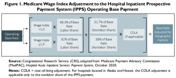
HWI was implemented in 1983 as a part of Medicare’s Inpatient Prospective Payment System (IPPS).[3] IPPS provides payments to most short-term, acute-care hospitals for services provided during a beneficiary’s inpatient stay under Medicare Part A. IPPS uses a base rate, calculated using hospital-reported costs, to determine pre-adjustment payment levels for two payments: the operating payment (for labor and supplies) and the capital payment (depreciation, interest, rent, and property-related insurance and taxes).[4] The IPPS operating and capital payments are the same for all hospitals and serve as the starting point for geographic, diagnostic, and other adjustments. Once determined, the operating base rate is then adjusted by the HWI, and that value is further adjusted by case mix and other factors before being converted to a dollar value. See Figure 1 for an illustration of how the operating base rate is adjusted for geographic factors. [5] The HWI is also used to adjust payments to other components of Medicare’s Part A services such as home health, hospice, ambulatory surgical services, and long-term care hospitals.

Calculation of Payments using HWI

As stated above, the HWI attempts to tailor payments to reflect the price of labor in a given geographic area. These geographic areas are referred by the Centers for Medicare & Medicaid Services (CMS) as core-based statistical areas (CBSAs). CBSAs are made up of metropolitan statistical areas (MSAs) and micropolitan statistical areas (non-MSAs). In practice, CMS assigns distinct HWI values to all MSAs and then a single HWI value to all of the non-MSAs in a state. For FY2021, CMS recognizes 590 geographic markets across the United States and its territories, with 517 being MSAs and the remaining 73 being non-MSAs.[6] The HWI for a geographic area is calculated as the AHW paid by all IPPS hospitals in that geographic area divided by the AHW paid by all IPPS hospitals nationwide.[7] This seemingly simple calculation is made up of a variety of interconnected parts that attempt to weight the data according to the occupation mix of a hospital. To produce an operating base rate adjusted for geographic factors, the HWI itself must be adjusted by the occupational mix with a factor known as the Occupational Mix Adjustment (OMA) before being added to a nonlabor portion of the payment. These elements are described in detail below.

Labor-related portion: In order to determine the HWI, the AHW for hospitals must be calculated using reported paid hours and the cost of wages.[8] To ensure that the HWI reflects the regional market price of labor and not the labor decisions of a hospital, a hospital’s AHW is adjusted based on the hospital’s occupational mix – the proportion of certain positions at the hospital relative to the proportion of those positions nationally. This proportion is the OMA. Due to limited data, only the nursing profession is used in determining a hospital’s OMA, specifically registered nurses, licensed practical nurses, surgical technologists, nurse assistants, orderlies, and medical assistants.

After calculating the OMA for hospitals’ AHW, data are aggregated for a geographic region and then divided by the national data to find the HWI for that geographic region. A hospital uses the HWI of its geographic region. The national average HWI is defined as 1.0000; regions with a higher-than-average AHW will have an HWI above 1.0000 and regions with a lower-than-average AHW will have an HWI below 1.0000. To find the labor portion of the geographically adjusted base operating rate, the HWI is multiplied by the labor share of the base operating payment. For areas with an HWI above 1.0000, Medicare defines the labor share as 68.3 percent of the base operating payment. For areas with an HWI equal to or below 1.0000, CMS defines the labor share as 62 percent of the base operating rate.

Nonlabor-related portion: In addition to labor expenses, hospital costs for supplies and other non-labor resources are adjusted by a Cost-of-Living Adjustment (COLA). The COLA is usually 1.0 unless a hospital is in Hawaii or Alaska, due to the unusually excessive costs of living in those states. Once the geographically adjusted labor and non-labor portions are determined, they are added together to provide the complete geographically adjusted operating base rate for a payment to a hospital. The geographically adjusted base rate is then adjusted for the Diagnosis Related Grouping weight to determine the final operating payment to a hospital.[9]

Issues with HWI

Given the HWI’s complexity and reliance on insufficient data, numerous complaints have been raised over the years about its fairness and accuracy. Most adjustments to the HWI over time have involved congressionally enacted rules allowing for the reclassification of hospitals to certain regions.[10] These actions do not, however, solve core issues at the heart of the HWI, including budget neutrality, labor mix issues, data limitations, geographic bias, and labor pricing issues, to name a few.  

Budget neutrality: As with many types of adjustments that affect Medicare rates, adjustments to HWI scores must be budget neutral. In practice, this requirement means that when one area’s HWI is increased, thereby increasing a hospital’s operating base rate, another area’s base rate is decreased. Budget neutrality ensures at least some measure of cost control, and with Medicare’s Hospital Trust Fund expected to be bankrupt by 2026, cost control is a worthy concern. This principle means, however, that even well-reasoned changes require robbing Peter to pay Paul.

Labor mix: As previously mentioned, the OMA only takes into account nursing professions, which account for less than half of hospital workers.[11] The majority of hospital professions are therefore represented by the hospital’s reported cost of labor, and not the local market price of labor. As such, while the intent of the HWI is to account for fair market prices and encourage efficient labor mixes, in practice more than half of the labor mix accounted for in HWI is based around the cost of labor. CMS’s occupational mix survey could be expanded to include more or even all occupations at a hospital, although this approach has the downside of potentially creating additional administrative burdens for hospitals.

Even a more inclusive occupational mix survey of hospitals would still fall short of capturing the market price of labor in a geographic area. As it stands, no part of the HWI accounts for the actual market price of labor for employment outside of the hospital. While physicians and more specialized occupations may have a relatively limited field of employment beyond hospitals, other occupations such as nurses and orderlies are frequently employed in the private sector by both health care and non-health care-related employers. The limited employment field used for HWI creates an inherent hospital-focused bias in the data. Additionally, hospitals employ a number of non-health care-specific employees – accountants, plumbers, electricians, carpenters, etc. – who can find work in non-health care markets. In particularly high-cost, competitive areas, individual hospitals may find its their labor costs far exceeding the regional AHW. Below, Figure 2 presents data on the cost margins in Medicare for certain high-cost regions compared to the national average. [12]

Figure 2. Medicare Margins by MSA for CY 2019

Source: Hospital Cost Report – RAND Corporation

Note: Critical access hospitals were excluded from the author’s calculation of the data. Data is from reporting periods from late-2018 through the end of CY 2019.

The graph above looks at the Medicare margins (meaning the percent of costs that Medicare payments cover) for short-term care hospitals in the United States, comparing the Medicare margins of hospitals in high-cost areas[13] to the national average Medicare margin. As the data show, Medicare does not fully cover costs in any of the areas or nationally with the Seattle and San Francisco MSAs having the worst margins at -27.7 percent and -41.2 percent, respectively.[14] The San Francisco MSA margin is over four times the national average. Meanwhile, Table 1 below displays the HWIs for similar statistical areas. [15]

Table 1. Hospital Wage Index for High-Cost Core Based Statistical Areas

National CBSA Average	0.9490[16]
Washington-Arlington-Alexandria, DC-VA-MD-WV CBSA	0.9994
Seattle-Bellevue-Kent, WA CBSA	1.1595
Boston, MA CBSA	1.2673
Average for High-Cost CBSAs	1.3196
New York-Jersey City-White Plains, NY-NJ CBSA	1.3468
San Francisco-San Mateo-Redwood City, CA CBSA	1.8251

As Table 1 indicates, despite a margin deficit four times that of the national average, the San Francisco-area HWI is just under twice the national average HWI. The Seattle area faces similar issues, with a margin deficit at three times the national average margin deficit but an HWI barely larger than the national average HWI. These figures indicates that the formula faces a mismatch in certain areas whose high costs of living may not be properly accounted for. There is a caveat to this conclusion: Hospital costs may be overstated due to the rising cost of care that is influenced by hospital consolidation and other non-geographic factors. Additionally, it has been found that hospitals who have their HWI readjusted to “better reflect” their costs are typically overcompensated, while those who do not readjust are typically undercompensated.[17]^,[18]

Hospital concentration: A study by the Robert Wood Johnson Foundation’s Health Care Cost Institute found that 72 percent of hospital markets surveyed were highly concentrated, meaning hospitals in a given area lacked competition, and more concentrated markets tended to be found in metro areas with 300,000 people or less. A 2010 survey found that 59 markets had only one hospital and 98 markets had only two hospitals, and almost all of those markets were small-to-medium markets.[19] There are numerous effects of hospital consolidation, and one of them is increased control over the AHW. If an area only has one hospital, the AHW is by default whatever that hospital is paying, further adding to the hospital-focused bias by limiting wage data to just a few employers.

Urban vs. rural concerns: As mentioned above, high-cost urban areas may find the HWI does not account for how much competition there is with other employers for labor and the necessary salary increases for cost-of-living. Conversely, the HWI also penalizes low-cost rural areas, who face the same staffing requirements as other hospitals but have an inherently lower volume of patients. AHWs in rural areas are inherently lower due to the lower cost of living and decreased competition for labor by employers. This means rural hospitals receive lower compensation – an intentional effect of geographic adjustment. IPPS as currently constructed incentivizes quantity, and even with the creation of quality-focused payment programs in recent years to de-emphasize quantity of services, the low volume of patients coupled with inherent labor requirements for hospitals means thin margins for rural hospitals. The Medicare margin in 2020 for rural hospitals (excluding critical access hospitals) was -6.6 percent.[20]

The HWI formula (see Fig. 1) does provide some tradeoffs in favor of lower-cost areas. Nonlabor costs are still linked to a given area’s cost of living and naturally will be higher in high-cost areas and lower in low-cost areas. In effect, the 38 percent of the adjusted base payment for the nonlabor share of hospitals with an HWI below 1.0000 may provide a higher relative payment to low-cost areas and further disadvantage high-cost areas that receive a lower relative payment for nonlabor costs despite the greater expense of the nonlabor portion.

There are several policy programs to address the issue of low payments to rural hospitals, including payment supports for critical access hospitals, rural referral centers, and sole community access hospitals.[21] Rural hospital closures have continued to increase over the last 15 years, however, with 181 closures since 2005. The factors behind these closures are not just linked to the HWI, but also a general heavy reliance on government payers (which pay lower rates than private insurers), decreasing rural populations, decreased utilizations of hospitals for health services, whether a state expanded Medicaid under the Affordable Care Act (ACA), and limited services due to a difficulty in attracting qualified practitioners, among other problems.

Geographic Practice Cost Indexes

Background

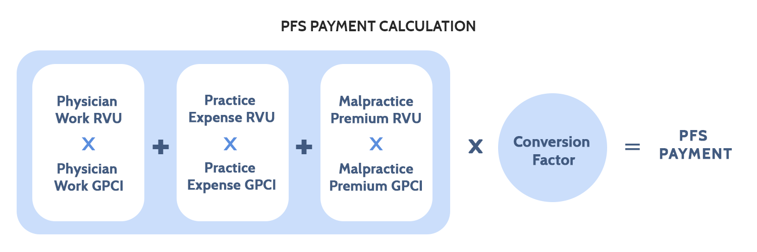
FFS Medicare payments to physicians and certain licensed clinical practitioners under the Physician Fee Schedule (PFS) are adjusted for geographic differences in the cost of business and living. In 1992, the basic methodology of the current PFS system, the Resource-Based Relative Value Scale (RBRVS), was established under the Omnibus Reconciliation Act of 1989.[22] The RBRVS attempts to make payments more equitable by basing payments on relative resource use (time, skill, supplies, etc.) and not historical prices, as well as reflecting local variation in input prices. The geographic areas used by the PFS are divided into 112 localities – 34 state-wide localities and 75 localities in the other 16 states.[23] The basic unit of the RBRVS is the relative value unit (RVU). RVUs represent the cost of resources for a given procedure relative to the cost of resources associated with a different procedure. A given number of RVUs are assigned to each Healthcare Common Procedure Coding System (HCPCS) code.[24] Each HCPCS code represents a specific procedure.[25]

GPCI and the PFS Calculation

RVUs and GPCIs: RVUs are the basis for payments. They are divided into three types: physician work (PW), practice expense (PE), and malpractice premium (MP) RVUs. Each type of RVU in an HCPCS code is adjusted by a corresponding GPCI and each HCPCS code is made up of a varying amount of the three types of RVUs. The GPCI values are based on the cost-share weights used in the Medicare Economic Index, which measures the average annual price change of a market basket of resources used to furnish services based on data from 2006.[26] These cost-share weights represent the percentage that PW, PE, and MP make of the total RVUs on average across all procedures – in 2020, the PW component comprised 50.866 percent of RVUs, the PE component comprised 44.839 percent of RVUs, and the MP component comprised 4.295 percent of RVUs.[27] It should be noted that each individual procedure is assigned a unique amount of each type of RVU. For example, an office code may be 40 percent PW RVUs, 57 percent PE RVUs, and 3 percent MP RVUs. 

Figure 3. PFS Payment Calculation

Physician Work: PW RVUs account for the time, effort, skill, judgement, and stress associated with a given service. These mostly subjective measures are determined by CMS with input from the American Medical Association/Specialty Society Relative Value Scale Update Committee, the Health Care Professionals Advisory Committee (HCPAC), the Medicare Payment Advisory Commission, other commentors, and medical literature, among other sources.[28] The PW GPCI is designed to reflect geographic differences in the cost of physician labor as compared to a national average.[29] The PW GPCI is based on the median earnings of seven nonphysician occupational categories (occupations with 5 or more years of college education) as reported by the Bureau of Labor Statistics Occupational Employment Statistics (BLS OES) reports from 2014-2017.[30] The range of the nonphysician occupational salaries is large and, due to political compromise, the adjustment has been limited to 25 percent of the total range of earnings above and below the national average. The 25 percent of the total range of nonphysician earnings in a given region is then divided by the national average to produce the PW GPCI. Since the passage of the ACA, there has been an artificial PW GPCI floor of 1.00, with Alaska receiving a floor of 1.50.[31] These floors have been extended multiple times and remain in place as of this writing.

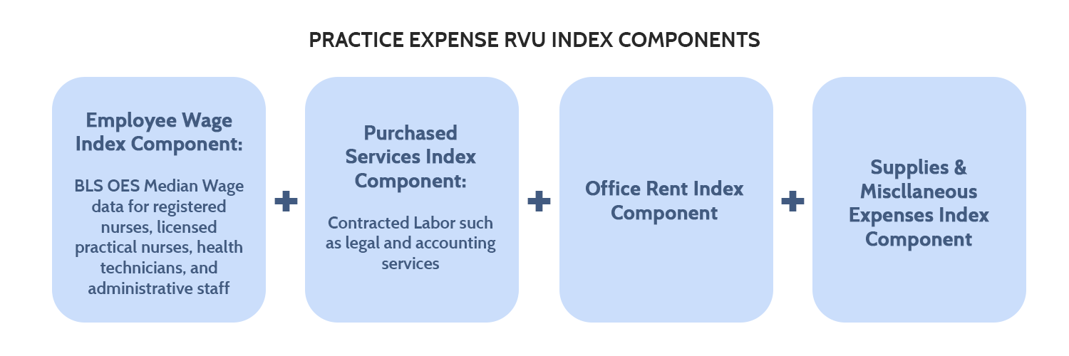
Practice Expense: The PE RVUs and their GPCI adjustments are made up of four index components: employee wages, purchased services, office rent, and other supplies and miscellaneous expenses.[32] There are two separate categories of PE RVUs, based on whether services were rendered in a facility (such as an ambulatory surgical center or hospital outpatient department) or a so-called “non-facility” (such as a physician’s office).[33] Facility payments are usually lower, as the facilities typically have certain supply and other costs built-in to their revenue model.

The employee wage index component measures the variation in the price of labor directly employed by a physician practice, while the purchased services index component measures the price of contracted labor – such as legal and accounting services. The employee wage index component for non-physician staff is based on median wage data from BLS OES for four occupations: registered nurses, licensed practical nurses, health technicians, and administrative staff. The purchased services index component is also geographically adjusted using data from the BLS OES. As the name implies, the office rent index component measures the variation in the price of rent for the space a physician practice uses. The supplies and miscellaneous expenses index component covers various medical equipment and other purchases, but these are assumed to be purchased through a mostly national market and thus are not subject to geographic variation, giving the miscellaneous index component a PE GPCI of 1.00.

Figure 4. Practice Expense RVU Index Components

For all four index components, the index component GPCI would be determined by taking the regional average data of the individual index component and dividing it by the national average data of that index component. See Figure 5 for an illustration of this.

Figure 5. Practice Expense GPCI Components

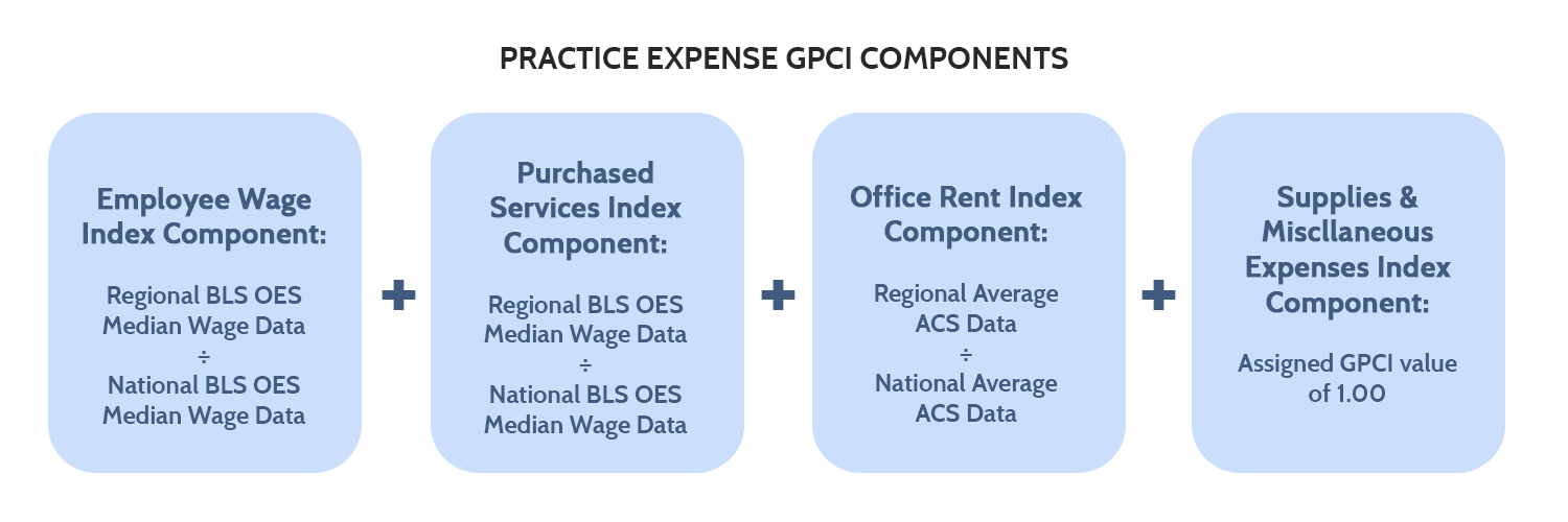
The employee wages and purchased services index components data are obtained through the wage data in the BLS OES reports from 2014-2017. The office rent portion data come from the five-year estimates of the American Community Surveys from 2013-2017. So-called “frontier states,” or states where 50 percent or more of their counties have a population per square mile of six people or less, have a PE GPCI cost floor of 1.00.[34]

Malpractice Premium: The MP RVUs are meant to represent the geographic differences in the costs of malpractice insurance.[35] The MP GPCI is calculated based on insurer filings of premium data for $1 million per incident and $3 million per year of mature claims-made policies. MP premiums vary heavily based on specialty and the state in which a physician practices. The geographic variation is due to state tort laws governing medical malpractice as well as the concentration of certain specialties in a given area. The main source for premium data is state rate filings.

Common Issues: All the GPCIs share common issues. For one, the calculation methodology has not been updated in decades; the 2011 Institute of Medicine (IOM) report that has been cited throughout this primer is still mostly accurate regarding payment methodology. For another, many of the assumptions made about wages and earnings are based on proxy occupations that may or may not reflect the actual value of the health care workforce.

Additionally, because the 112 GPCI geographic regions have only been updated once since their modern configuration in 1997, GPCI adjustments, which apply to Medicare Part B services, often lag behind their HWI counterparts in Part A.[36] This lag is due in part to the GPCI adjustments relying more on non-health care inputs to determine the adjustment factor. For example, San Jose, California, has the highest HWI in the nation at 1.8541, but a PW GPCI of 1.096 (also the highest PW GPCI in the nation). Santa Cruz, California, has the second highest HWI at 1.8486, but a PW GPCI of 1.042.[37] If Medicare has determined that hospitals in these areas need the higher geographic adjustment, it begs the question of why physicians and other Part B providers would not also need a similarly higher geographic adjustment?

Adding to the problem above is that physicians do not have the same cost-reporting requirements (in part to avoid a circularity issue in determining physician payments) that hospitals have, and so we do not know the full extent of Medicare margin deficits for physicians and other Part B services. Without understanding how far off Medicare payments are from actual costs, it is difficult to determine the scope of any existing payment problems. Anecdotally, low payments relative to the amount of work done have been cited by physicians as one reason behind the decrease in independent physician practices.[38]

The 112 localities themselves are an issue that a 2011 IOM report made clear needs reform. The 112 geographic regions for GPCIs, as compared to the 590 geographic regions for the HWI, provide for much less precise adjustments to a given area’s payment. The IOM report stated that the MSAs used for the HWI should be used for GPCIs, given that both hospitals and physician services face the same labor market.[39]

PW GPCI: There is significant debate over whether or not the PW GPCI adjustment should be raised, eliminated, or kept the same. If the procedure is the same, then the time, effort, skill, judgement, and stress are all the same and do not rely on what market the procedure was done in. Alternatively, wages of all employees vary based on region in response to such things as cost of living, so there’s an argument to be made that physician payments should vary as well. Additionally, physicians often are self-employed and have ownership interests in their practice. Therefore, the total earnings of a physician are not truly reflected in the payments they receive for services. The PW GPCI is also calculated via proxy, namely by using the relative median hourly earnings from seven nonphysician occupation categories. The limit to 25 percent of the total range of the earnings of the seven occupation categories was a political compromise. When initially calculated, the range “seemed” too large – hardly an objective standard on which to base payments.[40] The reason in the first place for the proxy calculation was to avoid a circularity issue; without the proxy, Medicare payments to physicians would otherwise be based on Medicare payments to physicians, but the use of proxy occupations (and the artificially limited range) casts doubt on how accurate these payments are. This “quarter work GPCI” factor also means 75 percent of the PW GPCI is effectively set to a national value of 1.0000. This in turn affects over 38 percent of the average total GPCI aggregate impacts on geographic adjustments – in other words, over 38 percent of the average geographically-adjusted payment is not truly geographically adjusted.

PE GPCI: The PE GPCI occupational mix was originally developed using the four highest-paid employee categories in physicians’ offices in 1983. As expected, physicians’ offices have changed over the last four decades, with more diverse occupational mixes, and it is likely that these occupations no longer represent the true occupational mix of physician offices. Geographic variations in occupational mixes exist but are not currently accounted for. The geographic variation in occupational mixes may have several causes, including available labor supply and physician specialty concentration. Another issue is that employment data by practice type do not exist, and the occupational mix based on practice type is highly variable for reasons not always related to geography; e.g. a radiologist is going to hire more technicians than a pediatrician. Additionally, the supplies and miscellaneous index component, which is set to a value of 1.0000, makes up 9.97 percent of the average total geographically-adjusted payment. Combined with the PW GPCI, which makes up 38 percent of total geographically-adjusted payment, nearly half of the geographically-adjusted payment is not affected by local cost inputs.

MP GPCI: The MP GPCI has presented few challenges or issues and has received few complaints over the years, likely due to how small a share of the total payment it represents.

Conclusion

Medicare’s geographic adjustment of payments is a complex system of inputs, weights, and assumptions. The HWI provides for geographic adjustment of hospital payments through a calculation of the AHW in a given area as compared to the national AHW. GPCIs provide for geographic adjustment of physician payments through both hard numbers like office rent data and attempts to quantify intangible concepts such as the amount of stress a given procedure causes a physician. Both the HWI and GPCI geographic adjustments suffer from limited data and decades-old assumptions. There are no simple solutions for this flaw – and any solution would require massive data collection and sorting that could take years. Given the budget neutrality requirements for most changes in Medicare payments, payment recalculation will result in winners and losers, adding a political challenge to the budgetary and equity challenges. Nevertheless, some of these adjustment methods appear due for an update. A forthcoming paper will examine current proposals to alter geographic adjustment and specific options for doing so.

 

 

[1] Annual Medicare Trustees Report (2020): https://www.cms.gov/files/document/2020-medicare-trustees-report.pdf

[2] Geographic Adjustment in Medicare Payment: Phase I, Second Edition (2011): https://www.ncbi.nlm.nih.gov/books/NBK190074/

[3] Chapter 3: Hospital Wage Index – Geographic Adjustment in Medicare Payment: Phase I, Second Edition (2011): https://www.ncbi.nlm.nih.gov/books/NBK190066/

[4] Medicare Hospital Payments: Adjusting for Variation in Geographic Wages – CRS Report:  https://crsreports.congress.gov/product/pdf/R/R46702

[5] Medicare Hospital Payments: Adjusting for Variation in Geographic Wages – CRS Report:  https://crsreports.congress.gov/product/pdf/R/R46702

[6] Medicare Hospital Payments: Adjusting for Variation in Geographic Wages – CRS Report:  https://crsreports.congress.gov/product/pdf/R/R46702

[7] Chapter 3: Hospital Wage Index – Geographic Adjustment in Medicare Payment: Phase I, Second Edition (2011): https://www.ncbi.nlm.nih.gov/books/NBK190066/

[8] Medicare Hospital Payments: Adjusting for Variation in Geographic Wages – CRS Report:  https://crsreports.congress.gov/product/pdf/R/R46702

[9] Primer: The Inpatient Prospective Payment System and Diagnosis-Related Groups:  https://www.americanactionforum.org/research/primer-the-inpatient-prospective-payment-system-and-diagnosis-related-groups/

[10] Medicare Hospital Payments: Adjusting for Variation in Geographic Wages – CRS Report:  https://crsreports.congress.gov/product/pdf/R/R46702

[11] Note: The formula does not account for state and local nurse-to-patient ratio requirements. California is currently the only state to have a specified ratio requirement and this may negatively affect payments to California hospitals. https://www.nursingworld.org/practice-policy/nurse-staffing/nurse-staffing-advocacy/

[12]Hospital Cost Report – RAND Corporation: https://www.hospitaldatasets.org/data Note: Critical access hospitals were excluded from the author’s calculation of the data. Data is from reporting periods from late-2018 through the end of CY 2019.

[13] Cost of Living Index – The Council for Community and Economic Research:  https://www.coli.org/quarter-1-2021-cost-of-living-index-released-3-2-2-2/

[14] Note: California Health and Human Services reports the Medicare margin of San Francisco County to be -67.6 percent: https://data.chhs.ca.gov/dataset/hospital-annual-financial-data-selected-data-pivot-tables/resource/84d0a088-3689-40b4-ab82-6b04e8c0b213

[15] Note: Statistical areas in Table 1 are from Medicare wage index data, which uses different CBSA definitions than the Census Bureau MSAs used in Figure 2. As such, population areas are not exact matches and some discrepancies may exist. FY2021 Wage Index Home Page – CMS: https://www.cms.gov/Medicare/Medicare-Fee-for-Service-Payment/AcuteInpatientPPS/Wage-Index-Files-Items/FY2021-Wage-Index-Home-Page

[16] Note: By definition, the national average HWI is 1.0000. The reason for the discrepancy here is likely due to the exclusion of state-wide CBSAs from the Table 1 data.

[17] Medicare Hospital Payments: Adjusting for Variation in Geographic Wages – CRS Report:  https://crsreports.congress.gov/product/pdf/R/R46702

[18] Note: If a hospital has its HWI adjusted, the adjusted HWI applies only to IPPS payments, while the original HWI still applies to other Part A services.

[19] Chapter 3: Hospital Wage Index – Geographic Adjustment in Medicare Payment: Phase I, Second Edition (2011): https://www.ncbi.nlm.nih.gov/books/NBK190066/

[20] Medicare Reimbursement in Rural America – National Rural Health Association:  https://www.ruralhealthweb.org/NRHA/media/Emerge_NRHA/Advocacy/Policy%20documents/NRHA-Policy-Brief-Medicare-Reimbursement-in-Rural-America.pdf

[21] Chapter 3: Hospital Wage Index – Geographic Adjustment in Medicare Payment: Phase I, Second Edition (2011): https://www.ncbi.nlm.nih.gov/books/NBK190066/

[22] GPCI Timeline of Events – Geographic Adjustment in Medicare Payment: Phase I, Second Edition (2011):  https://www.ncbi.nlm.nih.gov/books/NBK190061/box/box_5_1/?report=objectonly

[23] Medicare CY 2020 Payment Policies Final Rule:  https://www.federalregister.gov/documents/2019/11/15/2019-24086/medicare-program-cy-2020-revisions-to-payment-policies-under-the-physician-fee-schedule-and-other#h-63

[24] HCPCS codes are based on the over 7,000 Current Procedural Terminology® (CPT) codes developed by the American Medical Association. Chapter 3: Hospital Wage Index – Geographic Adjustment in Medicare Payment: Phase I, Second Edition (2011) : https://www.ncbi.nlm.nih.gov/books/NBK190066/

[25] Chapter 5: Geographic Practice Cost Indexes – Geographic Adjustment in Medicare Payment: Phase I, Second Edition (2011): https://www.ncbi.nlm.nih.gov/books/NBK190061/

[26] Medicare Payment Advisory Commission 2021 Report to Congress: http://medpac.gov/docs/default-source/reports/mar21_medpac_report_to_the_congress_sec.pdf

[27] Medicare CY 2020 Payment Policies Final Rule:  https://www.federalregister.gov/documents/2019/11/15/2019-24086/medicare-program-cy-2020-revisions-to-payment-policies-under-the-physician-fee-schedule-and-other#h-63

[28] Medicare CY 2021 Payment Policies Final Rule:  https://www.federalregister.gov/documents/2020/12/28/2020-26815/medicare-program-cy-2021-payment-policies-under-the-physician-fee-schedule-and-other-changes-to-part

[29] Chapter 5: Geographic Practice Cost Indexes – Geographic Adjustment in Medicare Payment: Phase I, Second Edition (2011): https://www.ncbi.nlm.nih.gov/books/NBK190061/

[30] Medicare CY 2020 Payment Policies Final Rule:  https://www.federalregister.gov/documents/2019/11/15/2019-24086/medicare-program-cy-2020-revisions-to-payment-policies-under-the-physician-fee-schedule-and-other#h-63

[31] Medicare CY 2020 Payment Policies Final Rule:  https://www.federalregister.gov/documents/2019/11/15/2019-24086/medicare-program-cy-2020-revisions-to-payment-policies-under-the-physician-fee-schedule-and-other#h-63

[32] Medicare CY 2020 Payment Policies Final Rule:  https://www.federalregister.gov/documents/2019/11/15/2019-24086/medicare-program-cy-2020-revisions-to-payment-policies-under-the-physician-fee-schedule-and-other#h-63

[33] Medicare CY 2021 Payment Policies Final Rule:  https://www.federalregister.gov/documents/2020/12/28/2020-26815/medicare-program-cy-2021-payment-policies-under-the-physician-fee-schedule-and-other-changes-to-part

[34] Medicare CY 2020 Payment Policies Final Rule:  https://www.federalregister.gov/documents/2019/11/15/2019-24086/medicare-program-cy-2020-revisions-to-payment-policies-under-the-physician-fee-schedule-and-other#h-63

[35] Chapter 5: Geographic Practice Cost Indexes – Geographic Adjustment in Medicare Payment: Phase I, Second Edition (2011): https://www.ncbi.nlm.nih.gov/books/NBK190061/

[36] Medicare PFS Locality Configuration – CMS: https://www.cms.gov/Medicare/Medicare-Fee-for-Service-Payment/PhysicianFeeSched/Locality

[37] 2021 GPCI Value Table – CompuGroup Medical: https://emds.com/gpci/

[38] Updated Data on Physician Practice Arrangements – American Medical Association: https://www.ama-assn.org/system/files/2019-07/prp-fewer-owners-benchmark-survey-2018.pdf

[39] Chapter 5: Geographic Practice Cost Indexes – Geographic Adjustment in Medicare Payment: Phase I, Second Edition (2011): https://www.ncbi.nlm.nih.gov/books/NBK190061/

[40] Chapter 5: Geographic Practice Cost Indexes – Geographic Adjustment in Medicare Payment: Phase I, Second Edition (2011): https://www.ncbi.nlm.nih.gov/books/NBK190061/